Solutions Manual©
to accompany
MATLAB for Engineering Applications, Fifth Edition
By
William J. Palm III
University of Rhode Island
Solutions to Problems in Chapter Three
Word Processors and Solution Files: A Warning
The built-in MATLAB Editor does not recognize symbols that are not on the standard keyboard. So if you cut-and-paste a file from such a processor into the Editor, the Editor may generate an error message if your file contains symbols not found on the standard keyboard. For example, the expression y = -2*x contains a minus sign created with the hyphen symbol, which is not the "true" minus sign created by an equation editor. A "true" minus sign will generate an error message if pasted into the MATLAB Editor, as will many other symbols and Greek letters.
Another source of error is a pair of single quotation characters, such as xlabel('x'). Some word processors will automatically convert such a pair to "smart quotes", as `x´, and this will also generate an error message in the MATLAB Editor. Also, three periods (. . .) are used to denote line continuation in the MATLAB Editor and some word processors will convert these into a single symbol that is not recognized by the Editor. So, to avoid such errors, use only symbols from the standard keyboard when creating files.
In this solutions manual we have tried to avoid using smart quotes, ellipses, and "true" minus signs in our MATLAB code, so that you may cut-and-paste our code into the MATLAB Editor. If we missed any, please let us know.
Test Your Understanding Problems
T3.1-1 The session is
>>x = [5:20:85];
>>y = [10:30:130];
>>log(x.*y)-(log(x)+log(y))
ans
1.0e-014 *
-0.0444 0 -0.1776 -0.1776 0.1776
which are essentially zero, so the identity is correct.
T3.1-2 The session is
>>x = sqrt(2+6i)
x =
2.0402 + 1.4705i
>>abs(x)
ans
2.5149
>>angle(x)
ans
0.6245
>>real(x)
ans
2.0402
>>imag(x)
ans
1.4705
T3.1-3 The session is
>>x = [0:0.4:2*pi];
>>exp(i*x)-(cos(x)+i*sin(x))
The answers are essentially zero, which demonstrates that the identity is correct.
T3.1-4 The session is
>>x = [0:0.4:2*pi];
>>asin(x)+acos(x)-pi/2
The answers are essentially zero, which demonstrates that the identity is correct.
T3.1-5 The session is
>>x = [0:0.4:2*pi];
>>tan(2*x)-2*tan(x)./(1-tan(x).^2)
The answers are essentially zero, which demonstrates that the identity is correct.
T3.1-6 The session is
>>x = [0:0.1:5];
>>sin(i*x)-i*sinh(x)
The answers are essentially zero, which demonstrates that the identity is correct.
T3.1-7 The session is
>>x = [-10:0.1:10];
>>asinh(x)-log(x+sqrt(x.^2+1))
The answers are essentially zero, which demonstrates that the identity is correct.
T3.2-1 The function is:
function [ V, A] = cube(L)
% Volume V and surface area A of a cube whose side length is L.
V = L.^3;
A = 6*L.^2;
end
The test case is:
>>[V,A] = cube(10)
V =
1000
A =
600
T3.2-2 The function is:
function [ V ] = cone(r,h)
% Volume of a cone of radius r and height h.
V = pi*h.*r.^2/3;
end
The test case is:
>>V = cone(5,30)
V =
785.3982
T3.2-3 The function file is
function y = f5(x)
y = exp(-0.2*x).*sin(x+2)-0.1;
end
You can plot the function to obtain solution estimates to use with fzero, or you can simply try values of x between 0 and 10. The session is
>>fzero(@f5,0)
ans
1.0187
>>fzero(@f5,4)
ans
4.5334
>>fzero(@f5,6)
ans
7.0066
So the solutions are x = 1.0187, 4.5334, and 7.0066.
T3.2-4 The function file is
function y = f6(x)
y = 1 + exp(-0.2*x).*sin(x+2);
end
You can plot the function to obtain solution estimates to use with fminbnd, or you can simply try values of x between 0 and 10. The session is
>>fminbnd(@f6,0,3)
ans
2.5150
>>f6(ans)
ans
0.4070
>>fminbnd(@f6,3,10)
ans
8.7982
>>f6(ans)
ans
0.8312
So the solutions are (x,y)=(2.5150, 0.4070) and (x,y)=(8.7982,0.8312).
T3.2-5 Refer to Example 3.2-2. Modify the function file given in the example to use an area of 200 square feet rather than 100. The function file is
function L = channel(x)
L = 200./x(1)-x(1)./tan(x(2))+2*x(1)./sin(x(2));
end
Because this problem is similar to Example 3.2-2, we can try the same guess as in the example. The session is
>>x = fminsearch(@channel,[20,1])
x =
10.7457 1.0472
The answer is d = 10.7457 ft and θ = 1.0472 radians, or 60 degrees.
End-of-Chapter Problems
3.1 The session is
>> x = [0:2];
>> y = -3+i*x;
>> abs(y)
ans
3.0000 3.1623 3.6056
>> sqrt(y)
ans
0 + 1.7321i 0.2848 + 1.7553i 0.5503 + 1.8174i
>> (-5-7i)*y
ans
5.0000 + 21.0000i 22.0000 + 16.0000 29.0000 + 11.0000i
>> y/(6-3i)
ans
-0.4000 - 0.2000i -0.4667 - 0.0667i -0.5333 + 0.0667i
3.2 The session is
>>x = -5-8i; y = 10-5i;
>>abs(x*y)
ans
105.4751
>>angle(x*y)
ans
-2.5930
>>abs(x/y)
ans
0.8438
>>angle(x/y)
ans
-1.6657
3.3 The session is
>>(180/pi)*atan2(8,5)
ans
57.9946
>>(180/pi)*atan2(8,-5)
ans
122.0054
>>(180/pi)*atan2(-8,5)
ans
-57.9946
>>(180/pi)*atan2(-8,-5)
ans
-122.0054
The answers are in degrees.
3.4 The session is
>>x = [0:0.5:5];
>>sinh(x)-((exp(x)-exp(-x))/2)
ans
0 0 0 0 0 0 0 0 0 0 0
Because the results are all zero, the identity is correct for the given values of x.
3.5 The session is
>> x=linspace(1,100,500);
>> acosh(x)-log(x+sqrt(x.^2-1))
The answers are essentially zero and the identity is correct for the given values of x.
3.6 The script file is
epsilon = 8.854e-12;
L = 1; r = 0.001;
d = input('Enter a value for d in meters:')
C = pi*epsilon*L./log((d-r)./r);
disp('The capacitance in farads is: ')
disp(C)
The test case with d = 0.004 gives C= 2.5319e-11.
3.7 The script file is
beta_deg = input('Enter a value for beta in degrees:');
% Convert to radians.
beta = (pi/180)*beta_deg;
mu = input('Enter a value for mu:');
F2 = input('Enter a value for force F2:');
F1 = F2*exp(mu*beta);
disp('The force F1 is:')
disp(F1)
The answer for beta = 130 degrees, F2 = 100, and μ = 0.3 is F1 =197.5217 N.
3.8 The function file is
function y = temp(x)
% Converts from Fahrenheit to Celsius.
y = (5/9)*(x-32);
A test session follows.
>>temp([32,212])
ans
0 100
3.9 The session is:
>>% Create the function.
>>fun = @(x) 0.3*x-sin(2*x);
>>% Plot the function.
>>xp = 0:0.001:4;
>>plot(xp,fun(xp))
The plot shows that a zero is near 1.356 and the global minimum is near 0.659. So continue the sessions as follows:
>>% Find the root.
>>x1 = fzero(fun,1.356)
x1 =
1.3606
>>x2 = fminbnd(fun,0,1)
x2 =
0.7101
3.10 The function file is
function t = time(h,v0,g)
% Computes time t to reach height h, with initial speed v0.
roots([0.5*g,-v0,h])
end
A test session follows.
>> time(100,50,9.81)
ans
7.4612
2.7324
The smaller value is the time to reach the height while ascending; the larger value is the time to reach the height while descending.
3.11 The function files are
function h = height(V,r)
h = (V-2*pi*r.^3/3)./(pi*r.^2);
end
function cost = tower(r)
h = height(1000,r);
cost = 1000*pi*r.*h+1400*pi*r.^2;
end
The session is:
>>optimum_r = fminbnd(@tower,0,100)
optimum_r =
6.0095
>>min_cost = tower(optimum_r)
min_cost =
2.4960e+05
>>optimum_h = height(1000,optimum_r)
optimum_h =
4.8076
So the optimum radius is 6.0075 m; the optimum height is 4.8076 m, and the minimum cost is $249,600.
3.12 From the geometry of the right triangle,

Thus

The area is

which can be solved for L.

The perimeter P is

The function file is
function [L, P] = field(W,A)
L = (A-W.^2/4)./W;
P = 2*L+W+2*W/sqrt(2);
end
The session is:
>>[L, P] = field(6,80)
The results are L = 13.3333 meters and total = 39.6519 meters.
3.13 a. From the geometry of the right triangle,
Thus
The area is
which can be solved for L.
The perimeter P is
Substituting for L gives

The file is
function [W,P,L] = angular_fence(A,Wmin,Wmax,d);
% Computes minimum perimeter P and required width W to enclose an area A.
% Wmin and Wmax define the range of guessed values for W.
% d is the spacing.
% Define the W vector.
W_guess = [Wmin:d:Wmax];
% Calculate the perimeter.
P_guess = 2*A./W_guess+W_guess/2+sqrt(2)*W_guess;
[min_perimeter,i_P_min]=min(P_guess);
W = W_guess(i_P_min);
P = min_perimeter;
L = A./W-W/4;
end
Answers for Wmin = 1, d = 0.01, and Wmax =50 are: W = 9.1400, L=6.4677, P=35.0014.
Part b continued on the next page.
Problem 3.13 continued.
b. The following files are based on the equations in part a. They give the same answers as in part a, as they should.
function [P] = perimeter(W)
A = 80;
P = 2*A./W+W/2+sqrt(2)*W;
end
function [P,W,L] = dimensions(A,Pmin,Pmax)
optimum_W = fminbnd(@perimeter,Pmin,Pmax);
W = optimum_W;
P = perimeter(W);
L = A./W-W/4;
end
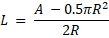
3.14 The area is found from

Solve for L:
The function file is:
function [ R,L, C ] = curved_fence(A, c1, c2, R1,R2,d);
R_guess=[R1:d:R2];
L_guess = (A-0.5*pi*R.^2)./(2*R);
C_guess = c1*(2*R_guess+2*L_guess)+c2*pi*R_guess;
[C, i_C_min]=min(C_guess);
R=R_guess(i_C_min)
L=L_guess(i_C_min)
end
where A is the area, c1 and c2 are the cost factors, R1 and R2 specify the low and high end of the guessed range for the radius, and d is the spacing used (here d = 0.1 foot).
The session is
>> [ R,L, C ] = curved_fence(2000, 40, 50, 1,50,0.1)
R =
21.4000
L =
29.9215
C =
7.4672e+03
R =
18.6000
L =
28.4023
C =
5.1575e+03
The optimum radius is 21.4000 feet, and the corresponding length is 29.9215 ft. The minimum cost is $74,672.
3.15 The area is found from
Solve for L:
The function file is
function cost = fence(R)
A = 2500;
L = (A-0.5*pi*R.^2)./(2*R);
cost = 50*(2*R+2*L)+60*pi*R;
The session is
>>optimum_R = fminbnd(@fence,0,100)
optimum R =
24.4001
>>min_cost = fence(optimum_R)
min_cost =
1.0246e+04
>>A = 2500;
>>optimum_L = (A-0.5*pi*optimum_R.^2)./(2*optimum_R)
optimum_L =
32.0656
The optimum radius is 24.4001 feet, and the corresponding length is 32.0656 feet. The minimum cost is $10,256.
3.16 The function files are
function deltaV = volume(t)
global r x
V = 1e+9+1e+8*(1-exp(-t/100))-r*t;
deltaV = V-0.01*x*1e+9;
function time = decrease(x,r)
global r x
time = fzero(@volume,1);
The session is
>>time = decrease(50,1e+7)
time =
54.1832
Thus it will take about 54 days.
3.17 a.

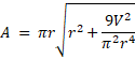
b. The function file is
function A = area(r)
global V
A = pi*r.*sqrt(r.^2+9*V.^2./(pi^2*r.^4));
c) First plot the area versus r to locate the minimum approximately. It is between r=1 and r=3. The session is
>>global V
>>V = 10;
>>r = [0.5:0.01:5];
>>plot(r,area(r))
>>[r, A] = fminbnd(@area,1,3);
>>h = 3*V/(pi*r^2)
The results are r = 1.8901, A = 19.4393, and h = 2.6730. Plotting A versus r shows that A is 10% above its minimum value when r is approximately 1.48 and 2.35.
3.18 a) The function is
function [V, A] = torus(a,b)
V = 0.25*pi^2*(a+b).*(b-a).^2;
A = pi^2*(b.^2-a.^2);
The session is
>>a = [0.25:0.01:4];
>>b = a+2;
>>[V,A] = torus(a,b);
>>subplot(2,1,1),plot(a,V),xlabel(’a (in.)’,ylabel(‘V (cu. in.)’)
>>subplot(2,1,2),plot(a,A),xlabel(‘a (in.)’),ylabel(‘A (sq. in.)’)
The plot follows.
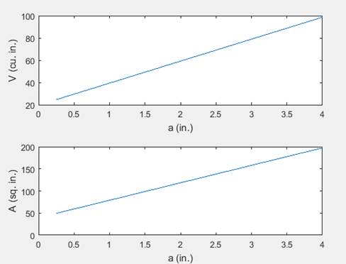
Figure for Problem 3.18
3.19 The function is
function [a,b,c,d] = cubicpoly(x,y)
for k = 1:4
A(:,k) = x.^(4-k);
end
B = y’;
coeff = A\B;
a = coeff(1);
b = coeff(2);
c = coeff(3);
d = coeff(4);
end
The session is
>>x = [-2,0,2,4];
>>y = [-20,4,68,508];
>>[a,b,c,d] = cubicpoly(x,y)
>>p=[a,b,c,d]
a =
7
b =
5
c =
-6
d =
4
>>polyval(p,x)
ans =
-20 4 68 508
This verifies that the answers are correct. The polynomial is

3.20 The function is
function []= savings_balance(N,A,r)
% Solution to Problem 3.19
format bank
n=1:N;
B=A*(1+r/100).^n;
Table=[n' B'];
disp(' Year Balance')
disp(Table)
format short
end
The test session is:
>>savings_balance(10,1000,3.5)
Year Balance
1.00 1035.00
2.00 1071.22
3.00 1108.72
4.00 1147.52
5.00 1187.69
6.00 1229.26
7.00 1272.28
8.00 1316.81
9.00 1362.90
10.00 1410.60
3.21 The function is:
function [] = ellipse_plot(a,b)
% Plots one ellipse.
x = linspace(-a,a,200);
y1 = sqrt((1-x.^2/a^2).*b^2);
y2 = -sqrt((1-x.^2/a^2).*b^2);
plot(x,y1,x,y2,xlabel('x'),ylabel('y')
end
The test case is:
>>ellipse_plot(1,2)
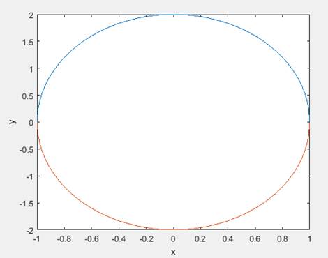
Figure for Problem 3.20
3.22 a. Try plotting with several upper limits on x. You will find that there are two zeros between 0 and 1.5.
b. The function is
function y = fex(u)
y = 1-7*u.*exp(-2*u);
end
From part a we use [0, 1.5] as the range. The session is:
>> fzero(@fex, [0, 1.5])
We get the message:
Error using fzero (line 274)
Function values at the interval endpoints must differ in sign.
So, we try
fzero(@fex, [0, 0.5])
ans =
0.2233
So, the zero is at x = 0.2233. Then we try:
fzero(@fex, [0.5, 1.5])
ans =
0.9443
So, the second zero is at x = 0.9443.
3.23 Substituting the given parameter values and subtracting the exponential from the logistic function, we obtain
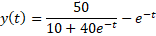
So we look for a value of t that makes y(t) zero. Create the following function.
function y = f23(t)
% Logistic minus exponential.
y = (50./(10+40*exp(-t))-exp(0.1*t));
end
Plotting y shows that a zero occurs between 0 and 50, so the session is:
>> fzero(@f23,50)
ans =
16.0944
>> 10*exp(-0.1*ans)
ans =
2.0000
The population size predicted by both models is 2 at t =
16.0944.
3.24 The session is
>>ex = @(x) 10*exp(-2*x);
>>x = [0:0.01:2];
>>plot(x,ex(x)),xlabel('x'),ylabel('10e^{-2x}')
The plot is shown below.
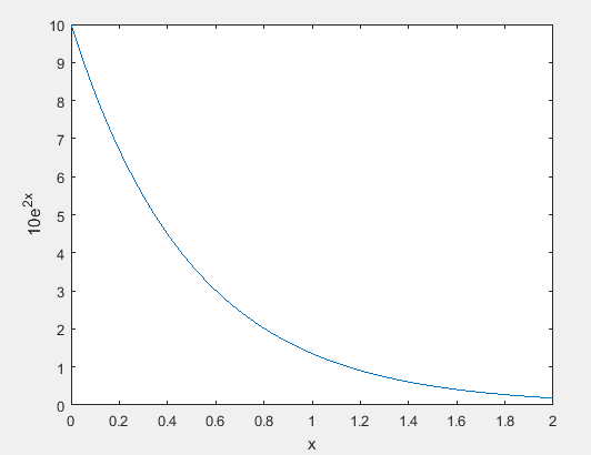
Figure for Problem 3.24
3.25 The session is
>>fn = @(x) 30*x.^2-300*x + 4;
>>x = [4:0.01:6];
>>plot(x,fn(x)),xlabel('x'),grid
Several plots show that the minimum occurs between x = 3 and x = 6. So, the session continues as follows:
>>[x, fval] = fminbnd(fn,3,6)
The answers returned are x = 4.1667, which is the location of the minimum value, and fval = -516.8333, which is the value of the minimum.
3.26 The script file is
f = @(x) x.^2;
g = @(x) 3*cos(x);
h = @(x) 6*exp(x);
u = @(x) h(g(f(x)));
x = [0:0.01:4];
plot(x,u(x)),xlabel('x'),ylabel('h')
The plot is shown below.
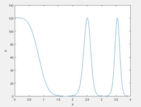
Figure for Problem 3.26
3.27 Create the following function file.
function f = cubic(a,b,c,d)
f = @p;
function y = p(x)
y = a*x.^3+b*x.^2+c*x+d;
end
end
The session is
>> f = cubic(5,-14,-40,90);
>>x = [-5:0.01:5];
>>plot(x,f(x)),grid
>>fzero(f,-4)
ans =
-2.6828
>>fzero(f,2)
ans =
1.8437
>>fzero(f,5)
ans =
3.6391
The three zeros are located at x=-2.6828, 1.8437, and x=3.6391.
3.28 Create the following function file.
function f = parabola(a,b,c)
f = @p;
function y = p(x)
y = a*x.^2+b*x+c;
end
end
The session is
>>f = parabola(20,-200,12);
>>[x,fval] = fminbnd(f,0,10)
The returned answers are x = 5, which is the location of the minimum, and fval = -488, which is the value of the minimum.
3.29 The
session is:
>>% Create a parameterized function.
>>parfun = @(x,a) x.^4-5*x.^3+4*x.^2+2*x.*sin(a*x-4*a)+7;
>>% Set parameter value.
>>a = pi;
>>% Create a function of x alone.
>>fun = @(x) parfun(x,a);
>>% Plot the function.
>>xp = 0:0.001:4;
>>plot(xp,fun(xp)),xlabel(‘x’),ylabel(‘f(x)’)
The plot shows that a zero is near x = 1.6 and a minimum is near x = 3.37. Continue the session as follows.
>>% Find the root.
>>x1 = fzero(fun,1.6)
x1 =
1.6357
>>x2 = fminbnd(fun,0,4)
x2 =
3.3755
3.30 First create the function sse_quadratic.
function sse = sse_quadratic(x,tdata,ydata)
% Fit a quadratic y = at^2 + bt + c
a = x(1);
b = x(2);
c = x(3);
sse = sum((ydata-a*tdata.^2-b*tdata+c).^2);
end
The rest of the program follows.
tdata = 0:2:10;
ydata = [6,13.1,34,75,139,202];
fun_quadratic = @(x)sse_quadratic(x,tdata,ydata);
x0 = [1,1,1];
coeffs = fminsearch(fun_quadratic,x0);
tp=0:0.001:10;
y=coeffs(1)*tp.^2+coeffs(2)*tp+coeffs(3);
plot(tp,y, tdata,ydata,'o')
The coefficients a, b, c are
coeffs = 2.0174 -0.1927 -5.1750
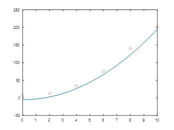
Figure for Problem 3.30
3.31 First create the function sse_logistic.
function sse = sse_logistic(x,tdata,ydata)
% Fit a logistic y = c/(1 + a*exp(-b*t))
a = x(1);
b = x(2);
c = 100;
sse = sum((ydata- c./(1 + a*exp(-b*tdata))).^2);
end
The rest of the program follows.
tdata = 0:1:15;
ydata = [13,16,20,25,31,39,45,49,55,63,69,77,82,86,89,92];
fun_logistic = @(x)sse_logistic(x,tdata,ydata);
x0 = [1,1];
coeffs = fminsearch(fun_logistic,x0);
tp=0:0.001:15;
c = 100;
yp = c./(1 + coeffs(1)*exp(-coeffs(2)*tp));
plot(tp,yp,tdata,ydata,'o')
The coefficients a and b are
coeffs = 6.9948 0.2817
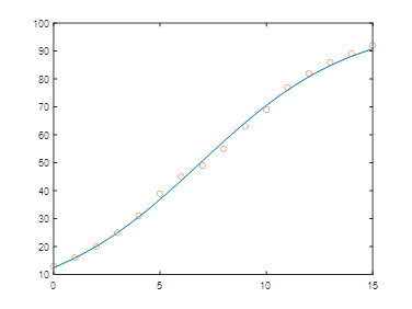
Figure for Problem 3.31
3.32 Assuming the data has been stored in the text file Prob3p28.txt, the session is
>>load Prob3p32.txt
>>A = Prob3p32;
>>mean(A)
The returned answers are 56.2500 44.2500 93.7500.
3.33 Assuming that the data have been saved in the Excel spreadsheet file Prob3p33.xls, the session is
>>A = xlsread('Prob3p33');
>>S = sum(A)
S =
227 169 377
The sums are 227, 169, and 377.
3.34 No MATLAB commands are needed to solve this problem.