Solutions Manual©

to accompany

MATLAB for Engineering Applications, Fifth Edition

William J. Palm III

University of Rhode Island

Solutions to Problems in Chapter Two

Word Processors and Solution Files: A Warning

The built-in MATLAB Editor does not recognize symbols that are not on the standard keyboard. So if you cut-and-paste a file from such a processor into the Editor, the Editor may generate an error message if your file contains symbols not found on the standard keyboard. For example, the expression y = -2*x contains a minus sign created with the hyphen symbol, which is not the "true" minus sign created by an equation editor. A "true" minus sign will generate an error message if pasted into the MATLAB Editor, as will many other symbols and Greek letters.

Another source of error is a pair of single quotation characters, such as xlabel('x'). Some word processors will automatically convert such a pair to "smart quotes", as `x´, and this will also generate an error message in the MATLAB Editor. Also, three periods (. . .) are used to denote line continuation in the MATLAB Editor and some word processors will convert these into a single symbol that is not recognized by the Editor. So, to avoid such errors, use only symbols from the standard keyboard when creating files.

In this solutions manual we have tried to avoid using smart quotes, ellipses, and "true" minus signs in our MATLAB code, so that you may cut-and-paste our code into the MATLAB Editor. If we missed any, please let us know.

Test Your Understanding Problems

T2.1-1 The session is

>>B = [2,4,10,13;16,3,7,18;8,4,9,25;3,12,15,17];

>>A=[B;B']

>>A(5,3)

T2.1-2 a) The session is

>>B = [2,4,10,13;16,3,7,18;8,4,9,25;3,12,15,17];

>>[x,k] = max(B);

>>[maxB,column]=max(x)

maxB =

column

>>row=k(column)

row

b) Continue the above session as follows:

>>C = sort(B)

C =

2 3 7 13

3 4 9 17

8 4 10 18

16 12 15 25

T2.3-1

>> x = [6,5,10]; y = [3,9,8];

>> s = x+y;

>> w = x.*y;

>> z = y.*x

Answers a. s = [9, 14, 18] b. w= [18, 45, 80] c. z= [18, 45, 80]. The same.

T2.3-2

>>A=[6,4;5,3]; B=[5,2;7,9];

>>S = A+B;

>>w = A.*B;

>>z = B.*A;

Answers a. S = [11, 6; 12, 12] b. w= [30, 8; 35, 27] c. z= [30, 8; 35, 27]. Yes.

T2.3-3

>>x=[6,5,10];

>>y=[3,9,8];

>>w=x./y;

>>z=y./x;

Answers a. w=[2, 0.5556, 1.25] b. z=[0.5, 1.8, 0.8]

T2.3-4

>>A=[6,4;5,3];

>>B=[5,2;7,9];

>>C=A./B;

>>D=B./A;

>>E=A.\B;

>>F=B.\A;

Answers. a. C=[1.2, 2; 0.7143, 0.3333] b. D=[0.8333, 0.5; 1.4, 3] c. E= [0.8333, 0.5; 1.4, 3] d. F=[1.2, 2; 0.7143, 0.3333] e. C and F are the same; D and E are the same.

T2.3-5 a) The session is

>>A = [21,27;-18,8];B = [-7,-3;9,4];

>>A.*B

ans

-147 -81

-162 32

>>A./B

ans

-3 -9

-2 2

>>B.^3

ans

-343 -27

729 64

T2.4-1

>>x=[6;5;3];

>>y=[2,8,7];

>>w=x*y;

>>z=y*x;

Answers. a. w=[12, 48, 42; 10, 40, 35; 6, 24, 21] b. z=73, obviously no!

T2.4-2 The session is

>>u = [6,-8,3]; w = [5,3,-4]

>>u*w'

ans

-6

T2.4-3 The session is

>>A = [7,4;-3,2;5,9];B = [1,8;7,6]

>>A*B

ans

35 80

11 -12

68 94

T2.4-4 The session is:

>>A = [4,3;8,2];

>>b = [23;6];

>>x = A\b

x =

2.0000

5.0000

To check the answer, compute the right-hand sides:

>>A*x

ans

23 6

Thus the correct solution is x=2, y=-5.

T2.4-5 The session is

>>A = [4,-2;3,5];b = [16;-1]

>>x = A\b

x =

3.0000

-2.0000

To check the answer, compute the right-hand sides:

>>A*x

ans

16 -1

Thus the correct solution is x=3, y=-2.

T2.4-6 The session is:

>>A = [6, -4, 8; -5, -3, 7; 14, 9, -5];

>>b = [112; 75; -67];

>>x = A\b

x =

2.0000

-5.0000

10.0000

To check the answer, compute the right-hand sides:

>>A*x

ans

112 75 -67

Thus the correct solution is x=2, y=-5, and z=10.

T2.5-1 The session is

>>roots([1,13,52,6])

ans

-6.4406 + 2.9980i

-6.4406 - 2.9980i

-0.1189

>>poly(ans)

ans

1.0000 13.0000 52.0000 6.0000

T2.5-2 The session is

>>p1 = [20,-7,5,10];p2 = [4,12,-3]

>>conv(p1,p2)

ans

80 212 -124 121 105 -30

T2.5-3 The session is

>>p1 = [12,5,-2,3];p2 =[3,-7,4 ]

>>[q,r] = deconv(p1,p2)

q =

4.0000 11.0000

r =

0 0.0000 59.0000 -41.0000

T2.5-4 The session is

>>p1 = [6,4,0,-5];p2 = [12,-7,3,9]

>>ratio = polyval(p1,2)/polyval(p2,2)

ratio =

0.7108

Using the deconv command, the session is

>>p1 = [6,4,0,-5]; p2 = [12,-7,3,9]

>>[q,r] = deconv(p1,p2);

>>ratio = polyval(q,2)+polyval(r,2)/polyval(p2,2)

ratio =

0.7108

T2.5-5 The session is

>>x = -7:0.01:1;

>>plot(x,polyval([1,13,52,6],x)),xlabel('x'),ylabel('y')

T2.7-1 The script file is

student(1).name = 'John Smith';

student(1).number = '392771786';

student(1).email = 'smithj@myschool.edu';

student(1).tests = [67,75,84];

student(2).name = 'Mary Jones';

student(2).number = '431569832';

student(2).email = 'jonesm@myschool.edu';

student(2).tests = [84,78,93];

student(3).name = 'Alfred E. Newman';

student(3).number = '555123456';

student(3).email = 'NewmanA@myschool.edu';

student(3).tests = [55,45,58];

T2.7-2 The session is

>>student(3).tests(2) = 53;

T2.7-3 The session is

>>new_student = rmfield(student,'SSN')

End-of-Chapter Problems

2.1 a) Either x = [5:23/99:28] or x = linspace(5,28,100) will work.

b) Either x = [2.:0.2:14] or x=linspace(2,14,61)} will work.

c) Either x = [-2:1/7:5] or Either x =linspace(-2,5,50) will work.

2.2 a) Type x= logspace(10,1000,50); b) Type x=logspace(10,1000,20);

2.3 The session is

>>x = linspace(0,10,6);

>>A = [3*x;5*x-20]

A =

0 6 12 18 24 30

-20 -10 0 10 20 30

2.4 Use the transpose operator. The session is

>>x = linspace(0,10,6);

>>A = [3*x;5*x-20]'

A =

0 -20

6 -10

12 0

18 10

24 20

30 30

2.5 The session is

>>A = [3,7,-4,12;-5,9,10,2;6,13,8,11;15,5,4,1];

>>v = A(:,2);

>>w = A(2,:);

2.6 The session is

>>A = [3,7,-4,12;-5,9,10,2;6,13,8,11;15,5,4,1];

>>B = A(:,2:4);

>>C = A(2:4,:);

>>D = A(1:2,2:4);

2.7 The length is 3 for all three vectors. The following session computes the absolute values.

>>x = [2,4,7];

>>length(x)

ans

>>abs(x)

ans

2 4 7

>>y=[2,-4,7];

>>abs(y)

ans

2 4 7

>>z=[5+3i,-3+4i,2-7i];

>>abs(z)

ans

5.8310 5.0000 7.2801

2.8 The session is

>>A = [3,7,-4,12;-5,9,10,2;6,13,8,11;15,5,4,1];

>>min(A)

ans

-5 5 -4 1

>>max(A)

ans

15 13 10 12

>>min(A')

ans

-4 -5 6 1

>>max(A')

ans

12 10 13 15

2.9 The session is

>>A = [3,7,-4,12;-5,9,10,2;6,13,8,11;15,5,4,1];

>>B = sort(A)

B =

-5 5 -4 1

3 7 4 2

6 9 8 11

15 13 10 12

>>C = [sort(A')]'

C =

-4 3 7 12

-5 2 9 10

6 8 11 13

1 4 5 15

>>D = sum(A)

D =

19 34 18 26

>>E = sum(A')

E =

18 16 38 25

2.10 a) The session is

>>A = [1,4,2;2,4,100;7,9,7;3,pi,42];

>>B = log(A)

>>B(2,:)

The answers are 0.6931, 1.3863, and 4.6052.

b) Type sum(B(2,:)). The answer is 6.6846.

c) Type B(:,2).*A(:,1). The answers are 1.3863, 2.7726, 15.3806, 3.4342.

d) Type max(B(:,2).*A(:,1)). The answer is 15.3806.

e) Type sum(A(1,:)./B(1:3,3)'). The answer is 3.3391.

2.11 The script file is

A = [3,-2,1;6,8,-5;7,9,10];

B = [6,9,-4;7,5,3;-8,2,1];

C = [-7,-5,2;10,6,1;3,-9,8];

D(:,:,1) = A;

D(:,:,2) = B;

D(:,:,3) = C;

max(max(D))

max(max(max(D)))

While this file is run, it produces the results:

ans(:,:,1) =

ans(:,:,2) =

ans(:,:,3) =

ans

Thus the largest element in the first, second, and third layer is 10, 9, and 10 respectively. The largest element in the entire array

is 10.

2.12

>>x = [5,9,-3];y=[7,4,2];

>>S = x+y;

>>w = x.*y;

>>z = y.*x;

Answers. a. s=[12, 13, -1] b. w=[35, 36, -6] c. The same.

2.13

>>A = [9,6;2,7];B=[8,9;6,2];

>>w = A.*B;

>>z = B.*A;

Answers. a. w=[17, 15; 8, 9] b. z=[72, 54; 12, 14] c. Yes.

2.14

>>x = [10,8,3]y = [9,2,6];

>>w = x./y;

>>z = y./x;

Answers. a. w=[1.1111, 4, 0.5] b. z=[0.9, 0.25, 2]

2.15 The session is

>>A = [-7,11;4,9]; B = [4,-5;12,-2]; C = [-3,-9;7,8];

>>A+B+C

ans

-6 -3

23 15

>> A-B+C

ans

-14 7

-1 19

>>(A+B)+C

ans

-6 -3

23 15

>>A+(B+C)

ans

-6 -3

23 15

>> B+C+A

ans

-6 -3

23 15

>>A+C+B

ans

-6 -3

23 15

2.16

>>A = [5,9;6,2];B=[4,7;2,8];

>>C = A./B;

>>D = B./A;

>>E = A.\B;

>>F = B.\A;

Answers. a. C= [1.25, 1.2857; 3, 0.25] b. D=[0.8, 0.7778; 0.3333, 4] c. E=[0.8, 0.7778; 0.3333, 4] d. F=[1.25, 1.2857; 3, 0.2500] e. C and F are equal. D and E are equal.

2.17 The session is

>>A = [56,32;24,-16]; B = [14,-4;6,-2];

>>A.*B

ans

784 -128

144 32

>> A/B

ans

176 -168

-12 32

>> B.^3

ans

2744 -64

216 -8

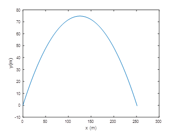
2.18 The script is

% Part a

v0 = 50;A = 50;g=9.81;

t_guess = input('Enter a guess for time to hit: ')

d = t_guess/1000;

t = [0:d:t_guess];

y =( v0*sind(A))*t-0.5*g*t.^2;

% y_max is the maximum height; t_max is the time to reach y_max.

[y_max,i_max] = max(y)

t_max = d*i_max

t_hit = 2*t_max

% Part b

clear t y

t = [0:d:2*t_max];

x = v0*cosd(A)*t;

y = (v0*sind(A))*t-0.5*9.81*t.^2;

plot(x,y),xlabel('x (m)'),ylabel('y (m)')

Enter a guess for time to hit: 10

t_guess =

y_max =

74.7736

i_max =

391

t_max =

3.9100

t_hit =

7.8200

Figure for Problem 2.18

2.19 The session is:

>>x = linspace(-2,16,300);

>>f=(4*cos(x))./(x+exp(-0.75*x));

>>plot(x,f),xlabel('x'),ylabel('y')

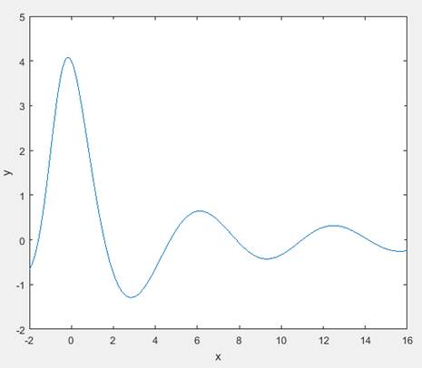
Figure for Problem 2.19

2.20 The session is:

>>x = linspace(-2*pi,2*pi,300);

>>f=3*x.*(cos(x)).^2-2*x;

>>plot(x,f),xlabel('x'),ylabel('y')

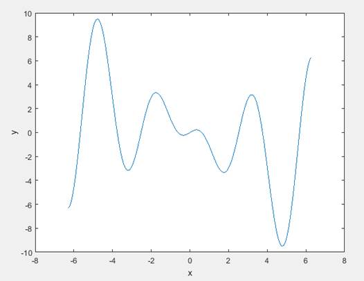
Figure for Problem 2.20

2.21 The session is:

>>x = linspace(-3.5,10,300);

>>f = 2.5.^(0.5*x).*sin(5*x);

>>plot(x,f),xlabel('x'),ylabel('y')

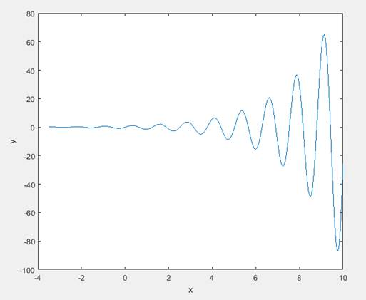
Figure or Problem 2.21

2.22 The session is:

>>x = linspace(-20,40,200);

>>y = (200-5*x)/6;

>>D = sqrt(x.^2+y.^2);

>>min_dist=min(D)

The answer is D = 25.6076 km.

2.23 The session is

>>F = [400,550,700,500,600]; D = [3,0.5,0.75,1.5,5];

>>W = F.*D

W =

1200 275 525 750 3000

>>Total_Work = sum(W)

Total_Work =

5750

The work done on each segment is 1200, 275, 750, and 3000 joules, respectively. (1 joule = 1 N m.) The total work done is 5750

joules.

2.24 Let the unit vectors i and j point east and north, respectively. Then the velocity of plane A is

and the velocity of plane B is v_B = –150i. The velocity of plane A relative to plane B is v_r = v_A – v_B. The session is as follows:

>>v_A = 300*[-cos(pi/4),-cos(pi/4)];

>>v_B = [-150,0];

>>v_R = v_A - v_B

v_R =

-62.1320 -212.1320

>>s_R = sqrt(v_R(1)^2 + v_R(2)^2)

s_R =

221.0439

The relative velocity is v_R = - 62.132i – 212.132j mi/hr. The relative speed is 221.0439 mi/hr. So Plane A is moving relative to plane B by 62.132 mi/hr to the west and 212.132 mi/hr to the south. The relative speed could also have been computed by s_R = sqrt(sum(v_R.*v_R)) or by s_R = sqrt(v_R*v_R').

2.25 The session is

>>wage = [5,5.5,6.5,6,6.25]; hours = [40,43,37,50,45];

>>output = [1000,1100,1000,1200,1100];

>>earnings = wage.*hours

earnings =

200.0000 236.5000 240.5000 300.0000 281.2500

>>total_salary = sum(earnings)

total_salary =

1.2582e+003

>>total_widgets = sum(output)

total_widgets =

5400

>>average_cost = total_salary/total_widgets

average_cost =

0.2330

>>average_hours = sum(hours)/total_widgets

average_hours =

0.0398

>>[maximum,most_efficient] = max(output./earnings)

maximum =

most_efficient =

>>[minimum,least_efficient] = min(output./earnings)

minimum =

3.9111

least_efficient =

The workers earned $200, $236.50, $240.50, $300, and $281.25 respectively. The total salary paid out was $1258.20, and 5400 widgets were made. The average cost to produce one widget was 23.3

cents, and it took an average of 0.0398 hr to produce one widget. The first worker, who produced 5 widgets per dollar of earnings, was the most efficient. The fifth worker, who produced 3.911 widgets per dollar of earnings, was the least efficient.

2.26 Let the unit vectors , , and point west, north, and down, respectively. Then the positions of the two divers are given by

The answer for (a) is given by |D₁|; for (b) by D = D₂ – D₁; and for (c) by |D|. The session is

>>D_1 = [-100,-30,40]; D_2 = [-30,-40,60];

>>magD_1 = sqrt(D_1*D_1')

magD_1 =

111.8034

>>D = D_2 - D_1

D =

70 -10 20

>>magD = sqrt(D*D')

magD =

73.4847

So diver 1 is 111.8034 ft from the starting point. To get to diver 2, diver 1 must swim 70 ft west, 10 ft south, and 20 ft up. To reach diver 2 in a straight line, diver 1 must swim 73.4847 ft.

2.27 The session is

>>force = [11,7,8,10,9]; k = [1000,600,900,1300,700];

>>x = force./k

x =

0.0110 0.0117 0.0089 0.0077 0.0129

>>energy = 0.5*k.*x.^2

energy =

0.0605 0.0408 0.0356 0.0385 0.0579

The unit for compression is a meter; the unit for energy is a joule.

2.28 The session is:

>>price = [300,550,400,250,500];

>>quantity = [5,4,6;3,2,4;6,5,3;3,5,4;2,4,3];

>> monthly_expenses = [price'.*quantity(:,1),price'.*quantity(:,2), price'.*quantity(:,3)]

monthly_expenses =

1500 1200 1800

1650 1100 2200

2400 2000 1200

750 1250 1000

1000 2000 1500

>>May_expenses = sum(monthly_expenses(:,1))

May_expenses =

7300

>>June_expenses = sum(monthly_expenses(:,2))

June_expenses =

7550

>>July_expenses = sum(monthly_expenses(:,3))

July_expenses =

7700

>>three_month_total = sum(monthly_expenses')

three_month_total =

4500 4950 5600 3000 4500

>>total = sum(three_month_total)

total =

22550

2.29 The script file is:

A = 2500;

R = [0.01:0.01:40];

L = (A-0.5*pi*R.^2)./(2*R);

cost = 40*2*(R+L)+50*pi*R;

[mincost,k] = min(cost);

Rmin = R(k)

Lmin = L(k)

mincost

The answers are:

Rmin = 23.9600, Lmin = 33.3521, mincost = $8348.60

2.30 The script file is:

r = [2:0.01:10];V = 500;

h = (V-2*pi*r.^3/3)./(pi*r.^2);

cost = 600*pi*r.*h+800*pi*r.^2;

plot(r,cost),xlabel('Radius (meters)'),ylabel('Cost ($)'), …

[radius,mincost] = ginput(1)

hmin = (V-2*pi*radius.^3/3)./(pi*radius.^2)

The plot is shown in the figure. The minimum cost is $91334. The optimum radius is 4.8915 m. The required height is 3.3909 m.

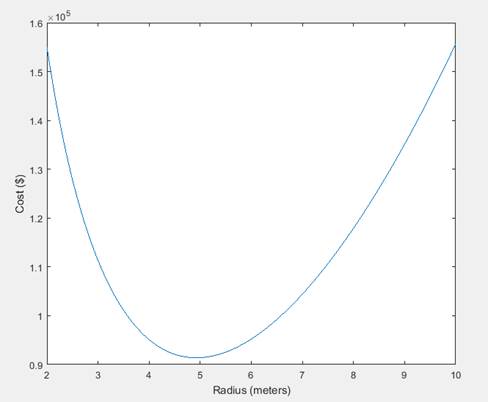
Figure for Problem 2.30

2.31 The MATLAB expressions are:

f = 1./sqrt(2*pi*c./x)

E = (x + w./(y + z))./(x + w./(y - z))

A = exp(-c./(2*x))./(log(y).*sqrt(d*z))

S = x.*(2.15 + 0.35*y).^1.8./(z.*(1-x).^y)

2.32 a) C(t) = 0.5C(0) implies that . Solve for : . The script file is:

k = [0.047:0.001:0.107];

thalf = -log(0.5)./k;

plot(k,thalf),xlabel('Elimination Rate Constant (1/hour)'), ylabel('Half-Life (hours)')

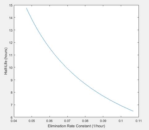
Figure for Problem 2.32a

Problem 2.32(b):

b) For and , . The script file is:

k = [0.047:0.001:0.107];

C = (1 - exp(-k))./k;

plot(k,C),xlabel('Elimination Rate Constant (1/hour)'),…

ylabel('Concentration (dimensionless)')

The plot is shown in the figure.

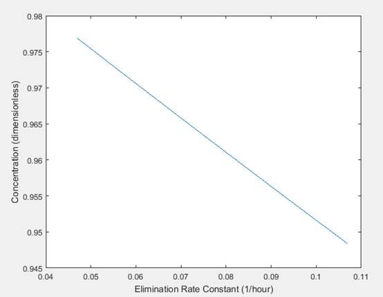
Figure for Problem 2.32b

2.33 a) The script file is

W = 100; Lb = 4; Lc = 6;

D = [0:0.01:Lb+1.5];

T = Lb*Lc*W./(D.*sqrt(Lc^2-D.^2));

[minT, k] = min(T)

minD = D(k)

minT = 133.3334, k = 425, minD = 4.2400

b) Append the following lines to the script file in part (a).

Dplot = [1.5:0.001:5.5];

upper = 1.1*minT

Tplot = Lb*Lc*W./(Dplot.*sqrt(Lc^2-Dplot.^2));

plot(Dplot,Tplot,[1.5, Lb + 1.5],[upper,upper]),grid,ginput(2)

The upper tension value is 1.1(133) = 146 N. The intersection of the two lines on the plot gives two solutions, which are approximately D = 3.26 m and D = 5.05 m.

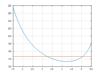Figure for Problem 2.33b

2.34 The session is:

>>x=[3;7;2];

>>y=[4,9,5];

>>w = x*y;

>>z = y*x;

Answers. a. w=[12, 27, 15; 28, 63, 35; 8, 18, 10] b. z=85. No.

2.35 The session is:

>>x = [3;7;2];

>>A = [2,6,5;3,7,4;8,10;9];

>>y = A*x;

>>z = x*A;

Answers. a. y=[58; 66; 112] b. Undefined product because inner dimensions are not equal.

2.36 The session is

>>A = [11,5;-9,-4]; B = [ -7,-8;6,2];

>>A*B

ans

-47 -78

39 64

>>B*A

ans

-5 -3

48 22

2.37 The session is

>>A = [4,-2,1;6,8,-5;7,9,10]; B = [6,9,-4;7,5,3;-8,2,1];

>>C = [-4,-5,2;10,6,1;3,-9,8];

>>A*(B+C)

ans

-31 -13 -7

173 147 -25

117 57 112

>>A*B+A*C

ans

-31 -13 -7

173 147 -25

117 57 112

>>(A*B)*C

ans

209 347 -136

297 -111 308

11207 562 250

>>A*(B*C)

ans

209 347 -136

297 -111 308

11207 562 250

2.38 For part (a) note that the first quarter material cost is computed by

7(16) + 3(12) +9(8) +2(14) + 5(13) = 326

and the second quarter material cost is computed by

7(14) + 3(15) + 9(9) + 2(13) + 6(16) = 346

and so on. Thus the quarterly costs can be computed by multiplying the transpose of the matrix of unit costs by the matrix of quarterly production volumes. The resulting matrix is quarterly_costs. Its first row contains the material costs, its second row contains the labor costs, and the third row contains the transportation costs. The four columns of quarterly_costs correspond to the four quarters. For part (b) the yearly costs for materials, labor, and transportation are found by summing the rows of quarterly_costs, or equivalently, by summing the columns of the transpose of quarterly_costs. For part (c) the total quarterly costs are found by summing the columns of quarterly_costs. The session is

>>unit_cost = [7,3,2;3,1,3;9,4,5;2,5,4;6,2,1];

>>quarterly_volume = [16,14,10,12;12,15,11,13;8,9,7,11;…

14,13,15,17;13,16,12,18];

>>quarterly_costs = unit_cost'*quarterly_volume

quarterly_costs =

326 346 268 364

188 190 168 214

177 186 160 204

>>yearly_costs = sum(quarterly_costs')

yearly_costs =

1304 760 727

>>total_quarter_cost = sum(quarterly_costs)

total_quarter_cost

691 722 596 782

(continued on the next page)

Problem 2.38 continued

The following table was created from the matrix quarterly_costs. All costs are in thousands of dollars.

Category	Quarter 1	Quarter 2	Quarter 3	Quarter 4
Materials	326	346	268	364
Labor	188	190	168	214
Transportation	177	186	160	204

From the vector yearly_costs we obtain the following information:

yearly materials cost = $1,304,000,

yearly labor cost = $760,000,

and

yearly transportation cost = $727,000.

From the vector total_quarter_cost we find that the total costs in each quarter are $691,000, $722,000, $596,000, and $782,000 respectively.

2.39 The amount of copper (Cu) needed to produce 1000 tons of each alloy is obtained by multiplying the Cu column in the table by 1000(0.01) = 10. (The 0.01 is needed to convert the table's percents into decimal values.) Thus we need 1000(0.01)(4.4+0+0+1.6+0) = 60 tons of copper. Extending this

method, we can see that we must multiply the matrix composition obtained from the table by a row vector consisting of five columns containing the value 10. The session is

>>composition = [4.4,1.5,.6,0,0;0,1,0,.6,0;0,1.4,0,0,4.5; …

1.6,2.5,0,0,5.6;0,.3,0,7,0];

>>alloy = 10*ones(1,5)

alloy =

10 10 10 10 10

raw_material = alloy*composition

raw_material =

60.0000 67.0000 6.0000 76.0000 101.0000

Thus we need 60 tons of copper, 67 tons of magnesium, 6 tons of

manganese, 76 tons of silicon, and 101 tons of zinc.

2.40 The script file is

%Enter the unit labor costs for the four products below.

labor1 = input('Enter the unit labor cost for product 1: ');

labor2 = input('Enter the unit labor cost for product 2: ');

labor3 = input('Enter the unit labor cost for product 3: ');

labor4 = input('Enter the unit labor cost for product 4: ');

u1 = [6, 2, 4, 9];u3 = [1, 4, 2, 3];

u2 = [labor1,labor2,labor3,labor4];

U = [u1', u2', u3'];

P = [10, 12, 13, 15;8, 7, 6, 4;12, 10, 13, 9;6, 4, 11,5];

C = U'*P;

Quarterly_Costs = sum(U'*P);

Category_Costs = sum((U'*P)');

disp('The cost for quarter 1 is: ')

disp(Quarterly_Costs(1))

disp('The cost for quarter 2 is: ')

disp(Quarterly_Costs(2))

disp('The cost for quarter 3 is: ')

disp(Quarterly_Costs(3))

disp('The cost for quarter 4 is: ')

disp(Quarterly_Costs(4))

disp('The materials cost is: ')

disp(Category_Costs(1))

disp('The labor cost is: ')

disp(Category_Costs(2))

disp('The transportation cost is: ')

disp(Category_Costs(3))

The results are (in thousands of dollars):

The cost for quarter 1 is: 444

The cost for quarter 2 is: 391

The cost for quarter 3 is: 558

The cost for quarter 4 is: 392

The materials cost is: 760

The labor cost is: 709

The transportation cost is: 316

2.41

A=[6,-3,4;12,5,-7;-5,2,6];

b=[41;-26;16];

x=A\b

x =

2.0035

-2.6848

5.2312

2.42 a.

A = [6,2,10;3,5,2;2,5,3];

b = [35;40;40];

x = A\b

x =

1.3571

6.6429

1.3571

P = 300*x(1) + 500*x(2) + 200*x(3)

P =

4000

b. Since the equations are linear, if we double the vector b, the solution x and the profit P will also double.

2.43 The position vector is r = [2, 10t+3, 0]. The session is

>>t = [0:.5:5];

>>P = [2*ones(1,length(t))',10*t'+3,zeros(1,length(t))];

>>location_5 = P(11,:)

location_5 =

2 53 0

>>v = [0,10,0];

>>L = 5*cross(P(11,:),v)

L =

0 0 100

The location of the mass at t = 5 s is given by the vector location_5. The location's coordinates are x =2, y = 53, z = 0 m. The angular momentum vector at t = 5 s is L = 0i + 0j + 100k. It lies entirely in the z direction, and has a magnitude of 100 kg m²/sec.

2.44 The session is

>>F = [12,-5,4];

>>r = [-3,5,2];

>>n = [6,5,-7];

>>M = dot(cross(r,F),n)

M =

8675

The magnitude is M = 675 N m.

2.45 The session is

>>A = [7, -3, 7]; B = [-6, 2, 3]; C = [2, 8, -8];

>>left = cross(A,cross(B,C))

left =

50 84 -414

>>right = B*dot(A,C)-C*dot(A,B)

right =

450 84 -414

So the left and right sides of the equation give identical results.

2.46 Note that we must express the vectors as three-dimensional vectors in order to use the cross-product. The session is

>>A = [5, 0, 0]; B = [1, 3, 0];

>>C = cross(A,B);

>>area = sqrt(C*C')

area =

The area is 15. If w had known that C has only one component ( C = [0, 0, 15]), we would not have needed to use the line area = sqrt(C*C')} to compute the area.

2.47 The session is

>>A = [5, 0, 0]; B = [2, 4, 0]; C = [3, 0, -2];

>>D = cross(B,C);

>>E = dot(A,D);

>>volume = abs(E)

volume =

The volume is 40. Note that since the dot product gives a scalar result, we can use the abs function to compute the magnitude of .

2.48

a = [6,9,4]; b = [-3,7,9];

cos_th = dot(a,b)/(norm(a)*norm(b));

th = acosd(cos_th)

th =

53.4351

The answer is in degrees.

2.49 The vector a is the vector from P to Q: a = [0, 1, 0][1, 0, 0] = [1, 1, 0], and the vector b is the vector from P to R: b = [0, 0, 1][1, 0, 0] = [1, 0, 1]. The MATLAB session is

>> a = [-1,1,0]; b = [-1,0,1];

>> c = cross(a,b);

>> d = norm(c);

>> area = 0.5*d

area =

0.8660

2.50 The session is

>>p1 = [3,-6,8,4,90];

>>p2 = [3, 5, -8, 70];

>>x = [-3:0.01:3];

>>y = polyval(p1,x);

>>z = polyval(p2,x);

>>plot(x,y,x,z,'--'),xlabel('x'),…

ylabel('y and z'),gtext('y'),gtext('z')

2.51 The session is

>>p = [3,-5,-28,-5,200];

>>x = [-1:0.01:1];

>>y = polyval(p,x);

>>plot(x,y,),xlabel('x'),ylabel('y'),grid,[x,y] = ginput(1)

The values returned at the peak are x = -0.0970 and y = 200.2190. These values are approximate because they depend on the placement of the cursor and the size of the plot. The exact value for the peak can be determined with calculus. It occurs at x = -0.0917.

2.52 The session is:

>>conv([5,0,-3,7,10],[4,-7,9,2])

ans =

20 -35 33 59 -36 -13 104 20

The answer is

2.53 The session is

>>[q,r] = deconv([5,-7,2,8],[6,3,-2])

q =

0.8333 -1.5833

r =

0 0 8.4167 4.8333

The answer is with a remainder of .

2.54 Using the deconv command, the session is

>>p1 = [36,-8,2]; p2 = [36, -5, 4, -3];

>>[q,r] = deconv(p1,p2);

>>ratio = polyval(q,5)+polyval(r,5)/polyval(p2,5)

ratio =

0.1963

2.55 The session is

>>conv([10,-9,-6,12],[5,-4,-12,8])

ans

50 -85 -114 272 -48 -192 96

The answer is .

2.56 The session is

>>[q,r] = deconv([14,-6,3,9],[5,7,-4])

q =

2.8000 -5.1200

r =

0.0000 0.0000 50.0400 -11.4800

The answer is 2.8x - 5.12 with a remainder of 50.04x – 11.48.

2.57 Using the deconv command, the session is

>>p1 = [24,-9,0,-7]; p2 = [10,5,-3,-7];

>>[q,r] = deconv(p1,p2);

>>ratio = polyval(q,5)+polyval(r,5)/polyval(p2,5)

ratio =

2.0458

2.58 Solving the ideal gas law gives V = RT/P. To solve the van der Waals equation for V, multiply both sides by V and collect terms to obtain a cubic equation for V:

The script file is:

P = 0.95;T = 300;R = 0.08206;a = 6.49;b = 0.0562;

ideal = R*T/P

Waals = roots([P,-(P*b + R*T),a,-a*b])

The answer for the ideal gas law is V = 25.9137. For the van der Waals model, V = 25.7047 (the other two roots are close to zero and are not physically significant).

2.59 a) The location of aircraft A is given by . The location of aircraft B is given by . The distance between them is given by . We can use the conv function as follows.

>>yB = [-160,410]; xA = [320, -800];

>>D2 = conv(xA,xA) + conv(yB,yB)

D2 =

128000 -643200 808100

Thus

Continue the session as follows:

>>t = [2:0.005:3];

>>D = sqrt(polyval(D2,t));

>>plot(t,D),xlabel('t'),ylabel('D'),grid,[x,y] = ginput(1)

The minimum distance determined from the graph is about D = 8.5 mi at about t = 2.51 hr after 1:00 P.M.

b) For , we must solve the equation

This is a second-order polynomial equation in the variable t. Continue the previous session as follows.

>>S = conv(xA,xA) + conv(yB,yB) - [0,0,900];

>>roots(S)

ans

2.5925

2.4325

The solutions are t = 2.5925 hr and t = 2.4325 hr after 1:00 P.M. At these two times the aircraft are 30 mi from each other.

2.60 The script file is

num = [3, -12, 20];

den = [1, -7, 10];

dt = 0.03;

x1 = [0:0.01:2-dt];

x2 = [2+dt:0.01:5-dt];

x3 = [5+dt:0.01:7];

y1 = polyval(num,x1)./polyval(den,x1);

y2 = polyval(num,x2)./polyval(den,x2);

y3 = polyval(num,x3)./polyval(den,x3);

plot(x1,y1,x2,y2,x3,y3),xlabel('x'),ylabel('y')

The range of y is determined by the value of dt. A small value of dt gives a large range for y , which makes the shape of the plot difficult to distinguish. Other choices besides dt = 0.03 will work. The plot is shown in the figure.

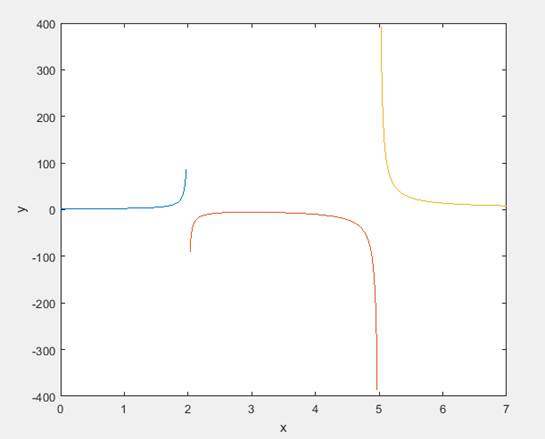
Figure for Problem 2.53

2.61 The script file is:

rho = 0.002378;S = 36;alpha=10;

V=[0:0.5:150]*(5280/3600);

CL = [4.47e-5,1.15e-3,6.66e-2,0.102];

CD = [5.75e-6,5.09e-4,1.81e-4,1.25e-2];

L = 0.5*rho*S*polyval(CL,alpha).*V.^2;

D = 0.5*rho*S*polyval(CD,alpha).*V.^2;

plot(V*(3600/5280),L,V*(3600/5280),D,'--'),...

title('Lift and Drag Versus Speed for \alpha = 10^o'),...

xlabel('Speed (miles/hour)'),…

ylabel('L, D (pounds)'),gtext('L'),gtext('D')

The plot is shown in the figure.

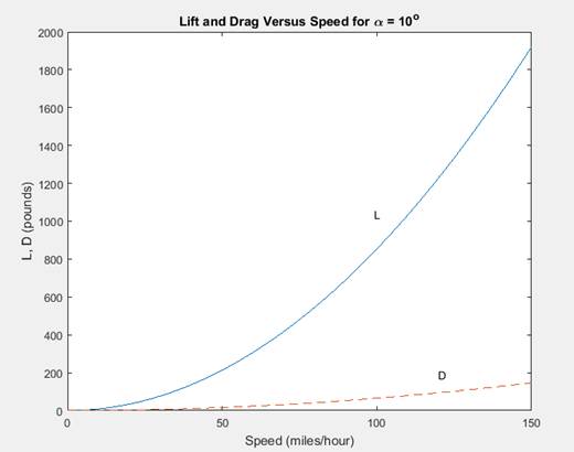
Figure For Problem 2.61

2.62 The script file is

rho = 0.002378;S = 36;

alpha = [-2:0.01:22];

CL = [4.47e-5,1.15e-3,6.66e-2,0.102];

CD = [5.75e-6,5.09e-4,1.81e-4,1.25e-2];

LoverD = polyval(CL,alpha)./polyval(CD,alpha);

plot(alpha,LoverD),xlabel('Angle of Attack \alpha (degrees)'),...

ylabel('Lift/Drag (dimensionless)')

The plot is shown in the figure.

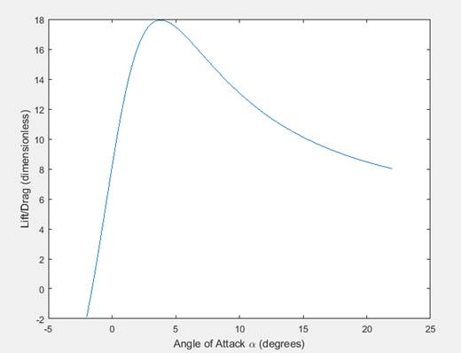
Figure for Problem 2.62

2.63 The script is

% Part a

v0 = 70;

A = 45;

g = 9.81;

t_hit = 2*v0*sind(A)/g

d = t_hit/1000;

t = [0:d:t_hit];

x = (v0*cosd(A))*t;

y = (v0*sind(A))*t-0.5*9.81*t.^2;

plot(x,y),xlabel('x (m)'),ylabel('y (m)')

% Part b

yd=100;

td=roots([g/2,-v0*sind(A),yd])

yd=200;

td=roots([g/2,-v0*sind(A),yd])

Answers. a. t_hit = 10.0912 s.

b. For , 7.2975 and 2.7938 s. These times correspond to the projectile passing 100 m going up and 100 m while descending. See the figure below.

For , . These are complex because the projectile never reaches 200 m, as shown by the figure below.

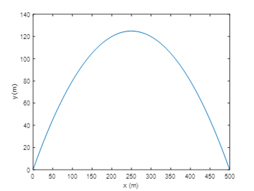
Figure for Problem 2.63

2.64 The script file is

% Using cell indexing:

A(1,1) = {'Motor 28C'};

A(1,2) = {'Test ID 6'};

A(2,1) = {[3,9;7,2]};

A(2,2) = {[6,5,1]};

% Using content indexing:

B{1,1} = 'Motor 28C';

B{1,2} = 'Test ID 6';

B{2,1} = [3,9;7,2];

B{2,2} = [6,5,1];

disp(B{2,1}(1,1))

When this file is run, it displays the answer 3.

2.65 Here we create a three dimensional cell array. The three layers correspond

to the values L = 1, 2, and 3 respectively. Some combinations of r and d values result in negative or infinite values for the capacitance C, and thus are invalid cases. The script file is

epsilon = 8.854e-12;

r1 = .001*[1,2,3]; r = [r1',r1',r1',r1'];

d1 = .001*[3,4,5,10]; d=[d1;d1;d1];

L = 1;

C{1,1,1} = 'L = 1';

C{1,2,1} = 'd';

C{2,1,1} = 'r';

C{2,2,1} = pi*epsilon*L./log((d-r)./r);

L = 2;

C{1,1,2} = 'L = 2';

C{1,2,2} = 'd';

C{2,1,2} = 'r';

C{2,2,2} = pi*epsilon*L./log((d-r)./r);

L = 3;

C{1,1,3} = 'L = 3';

C{1,2,3} = 'd';

C{2,1,3} = 'r';

C{2,2,3} = pi*epsilon*L./log((d-r)./r);

C{2,2,2}(1,3)

The structure of the array C can be seen by typing C. For the first layer you will see displayed:

C(:,:,1) =

' L = 1 ' 'd'

'r' [3x4 double]

The other two layers have a similar structure. To see the entire array, type celldisp(C).

The capacitance values are in the (2,2) cell in each layer. The values for are in the second layer (because L = 2 is the second value of L). The capacitance value C_ij corresponds to the values r_i and d_j. Thus the values for r = 0.001 and d = 0.005 are in the (1,3) element of the array in cell (2,2) (because r = 0.001 is the first value of r and d = 0.005 is the third value of d). The capacitance value is .

2.66 (a) One slug is the same as 14.594 kg. One pound is the same as 4.4482 N. One foot is the same as 0.3048 meter. The script file is named convert.m and is

%Convert slugs to kg

convert(1).mass = 14.594;

%Convert kg to slugs

convert(2).mass = 1/convert(1).mass;

%Convert lbs to newtons

convert(1).force = 4.4482;

%Convert newtons to lbs

convert(2).force = 1/convert(1).force;

%Convert feet to meters

convert(1).length = .3048;

%Convert meters to feet

convert(2).length = 1/convert(1).length;

(b) The session is

>>convert(1).length*70

ans

21.3360

>>convert(2).length*150

ans

492.1260

>>convert(2).force*48

ans

10.7909

>>convert(1).force*17

ans

75.6194

>>convert(1).mass*15

ans

218.9100

>>convert(2).mass*40

ans

2.7409

2.67 The script file is

bridge(1).location = 'Smith St';

bridge(1).maxload = 80;

bridge(1).yearbuilt = 1928;

bridge(1).duemaint = 2025;

bridge(2).location = 'Hope Ave';

bridge(2).maxload = 90;

bridge(2).yearbuilt = 1950;

bridge(2).duemaint = 2027;

bridge(3).location = 'Clark St';

bridge(3).maxload = 85;

bridge(3).yearbuilt = 1933;

bridge(3).duemaint = 2024;

bridge(4).location = 'North Rd';

bridge(4).maxload = 85;

bridge(4).yearbuilt = 1960;

bridge(4).duemaint = 2023;

2.68 The session is

>>bridge(3).duemaint = 2026;

2.69 The session is

>>bridge(5).location = 'Shore Rd';

>>bridge(5).maxload = 85;

>>bridge(5).yearbuilt = 1997;

>>bridge(5).duemaint = 2022;